Learning deep kernels for exponential family distributions
In our new paper, we tackle the problem of density estimation using an exponential family distribution with rich structure. The authors are me*, Dougal Sutherland*, Heiko Strathmann and Arthur Gretton
TL;DR
- We extend the kernel exponential family distributions using a deep kernel (kernel on top of network features);
- The deep kernel is trained by a cross-valiation like meta-training procedure;
- The train kernel is location-variant and adapts to local geometry of data distribution;
- We find that DKEF is able to capture the shape of distributions well.
Introduction
The goal is to fit a (non-)parametric distribution to observed data ${x}$ drawn from an unknown distribution $p_0(x)$. We know that an exponentialy family distribution can be written in the following form.
\[p_\theta(x)=\frac{1}{Z(\theta)}\exp[\theta \cdot T(x)]q_0(x)\]Many well known distributions (Gaussian, Gamma, etc.) can usually be written in this form, but we want to using a much more general parameterization. In our work, we take $\theta \cdot T(x) = f(x) = \langle f, k(x,\cdot) \rangle_{\mathcal{H}}$ where $f$ is a function in the reproducing kernel Hubert space $\mathcal{H}$ with kernel $k$, giving kernel exponential family. In short, we want to fit term inside the $\exp$ using a flexible function.
Learning such a flexible distribution in general using maximum likelihood (minimizing KL divergence) is challenging due to the intractable normalizer $Z$. However, an alternative objective is the score matching loss, which is related to the Fisher divergence. Thus, by minimizing the score matching loss, we are minimizing the Fisher divergence between $p_\theta$ and $p_0$. The sample-version score matching loss is
\begin{equation} \label{eq:score} J(\theta) = \sum_i\sum_d\partial_d^2\log p_\theta(x_i) + \frac{1}{2}(\partial_d\log p_\theta(x_i))^2 \end{equation} where $\partial_d^n$ is the $n$’th partial derivative w.r.t. the $d$’th dimension of $x_i$. The advantage for using score matching is that we can ignore the normalizer when optimizing the natural parameters $\theta$.
In order to use this approach to fit complex distributions, the kernel needs to adapt to the shapes at different parts of data domain. We show in Figure 1 of our paper that if we use a Gaussian kernel, and the kernel has only one length-scale, then even fitting a simple mixture of Gaussians can be challenging, whereas a location-variant kernel is able to capture the two scales and give a much better fit.
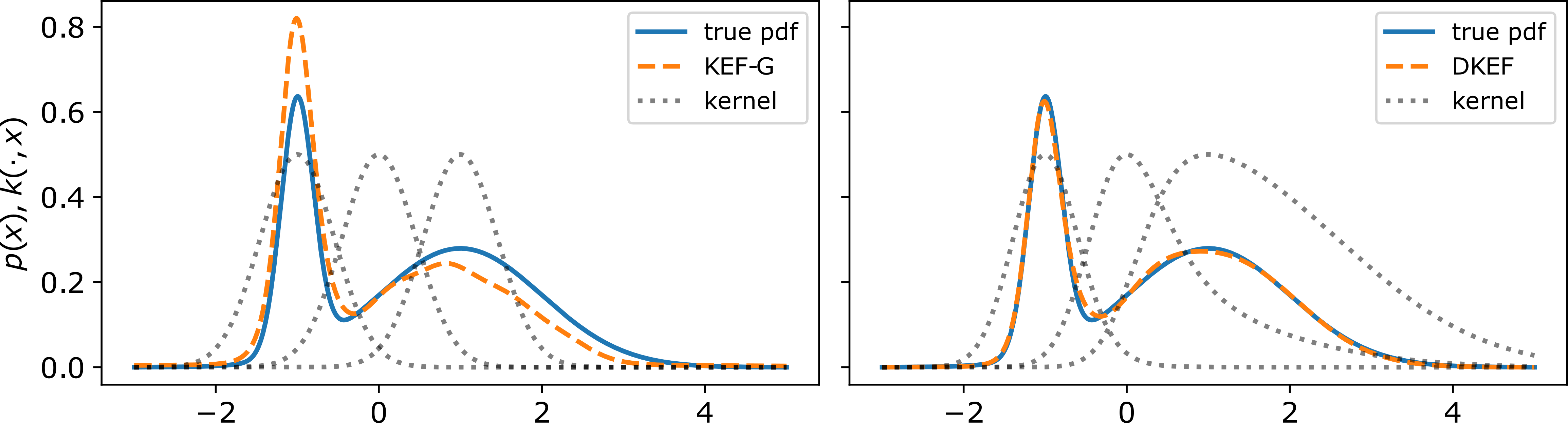 Fitting few samples from a Gaussian mixture,
using kernel exponential families.
Black dotted lines show $k(-1, \x)$, $k(0, \x)$, and $k(1, \x)$.
(Left) Using a location-invariant Gaussian kernel,
the sharper component gets too much weight.
(Right) A kernel parameterized by a neural network learns length scales that adapt to the density,
giving a much better fit.
Fitting few samples from a Gaussian mixture,
using kernel exponential families.
Black dotted lines show $k(-1, \x)$, $k(0, \x)$, and $k(1, \x)$.
(Left) Using a location-invariant Gaussian kernel,
the sharper component gets too much weight.
(Right) A kernel parameterized by a neural network learns length scales that adapt to the density,
giving a much better fit.
Deep kernel exponential family (DKEF)
In our work, we construct a flexible kernel using a deep neural network $\phi_w$ on top a Gaussian kernel
\[k(x,y)=\exp(-\frac{1}{2\sigma}\|\phi_w(x) - \phi_w(y)\|^2)\]or a mixture of such deep kernels above. We model the energy function as weighted sum of kernels centered at a set of inducing points $z$
\[f(x)=\sum_m\alpha_m k(x,z_m)\]The network $\phi(x)$ is fully connected with softplus nonlinearity. Using softplus ensures
- the energy is twice-differentiable and the score-matching loss is well defined;
- when combined with a Gaussian $q_0$, the resulting distribution is always normalizable (Proposition 2 in our paper).
Two-stage training (Section 3)
So far, the free parameters are the weights in the network $w$, $\alpha$, $\sigma$ and inducing points $z$. Naive gradient descent on the score objective will always overfit to the training data as the score can be made arbitrarily good by moving $z$ towards a data point and making $\sigma$ go to zero. Stochastic gradient descient might help, but would produce very unstable updates.
To train the model, we employ a two-stage training procedure which helps avoid overfitting and also enhances the quality of the fit, motivated by cross-validation. Consider a simpler scenario where we just use a simple Gaussian kernel with bandwidth $\sigma$ as our kernel, and minimize some loss (regression, classification, score maching, etc.). To find the optimal $\sigma$ (and any additional regularizers $\lambda$), one would do the following:
- first split the data into two sets $\mathcal{D}_1$ and $\mathcal{D}_2$;
- use the closed-form solution of the corresponding loss to find the linear coefficients $\alpha$ on (training) data $\mathcal{D}_1$,
- test the performance of the $\alpha$ on (validation) data $\mathcal{D}_2$.
- choose the optimal parameter that yeilds the minimum validation loss.
In the above procedure, one can think of $\alpha$ a function $\alpha(\sigma, \mathcal{D}_1)$, which is then validated on $\mathcal{D}_2$. What we really care is just the validation loss with $\alpha$ computed using parameter $\sigma$ and $\mathcal{D}_1$. We’d like to minimize it w.r.t. $\sigma$, which can be done using gradient descent. Note that this is possible as $\alpha$ is given by a closed-form solution on the training set.
Extending this approach to our model, we optimize not only $\sigma$ but also $w$ and $z$ (and regularization parameters) using the split-training procedure.
Experiments and evaluation
We first fit our model on a variety of synthetic distributions and compare with likelihood based normalizing-flows. Since we are using a different loss (score matching loss) than the others, different performances may be expected for different criterion, we thus compared different models using log likelihood and Fisher divergence. The results are in Figure 2 of the paper. In general, our model is able to fit the general shape of the distributions much better than likelihood based methods.
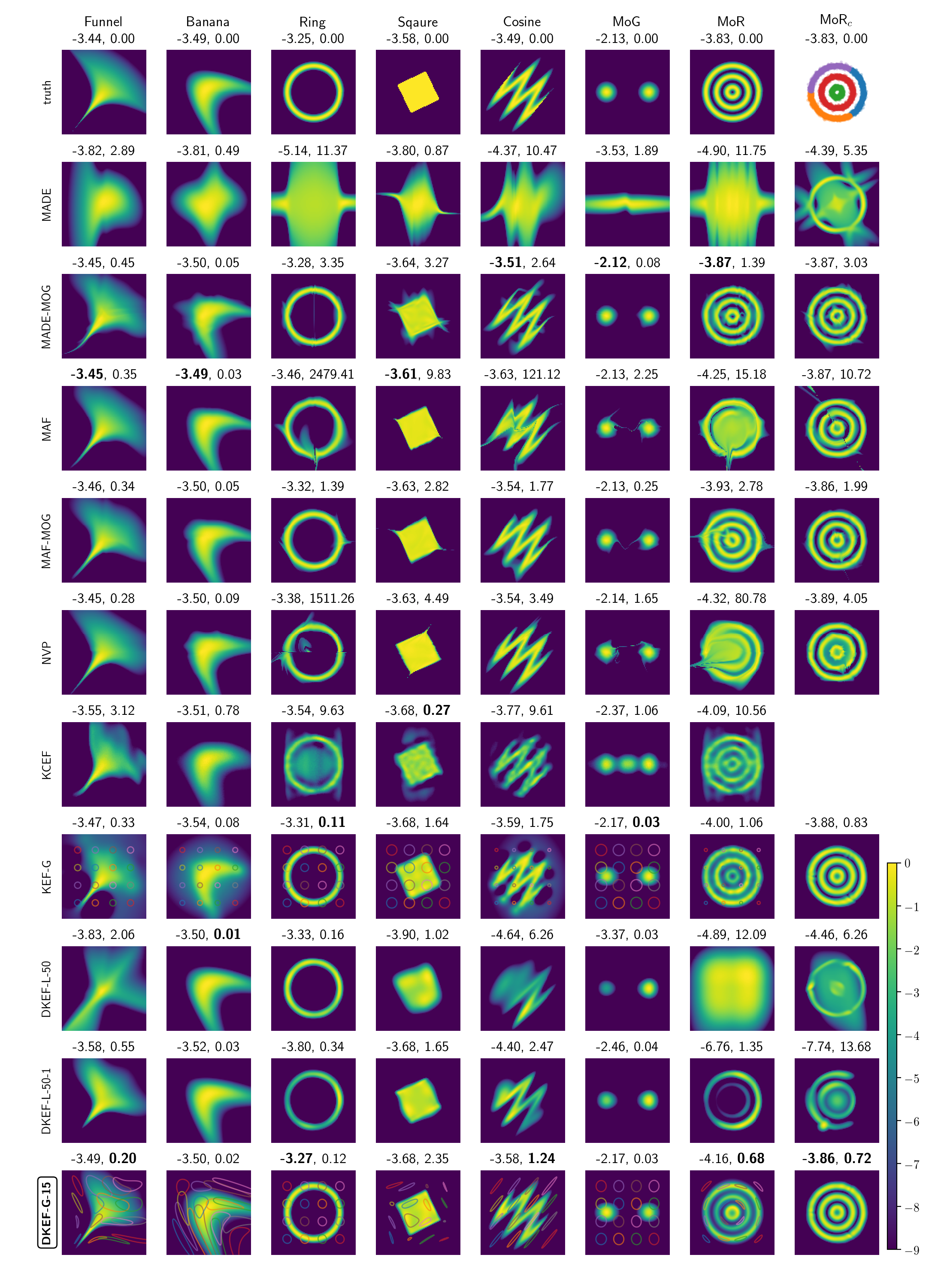 Log densities learned by different models. Our model is DKEF-G-15 at the bottom row.
Columns are different synthetic datasets. The rightmost columns shows a
mixture of each model (except KCEF) on the same clustering of MoR.
We subtracted the maximum from each log density, and clipped the minimum value at -9.
Above each panel are shown the average log-likelihoods (left) and Fisher divergence (right) on held-out data points.
Bold indicates the best fit.
For DKEF-G models,
faint colored lines correspond to contours at 0.9 of the kernel evaluated at different locations.
Log densities learned by different models. Our model is DKEF-G-15 at the bottom row.
Columns are different synthetic datasets. The rightmost columns shows a
mixture of each model (except KCEF) on the same clustering of MoR.
We subtracted the maximum from each log density, and clipped the minimum value at -9.
Above each panel are shown the average log-likelihoods (left) and Fisher divergence (right) on held-out data points.
Bold indicates the best fit.
For DKEF-G models,
faint colored lines correspond to contours at 0.9 of the kernel evaluated at different locations.
On real datasets, we compared models using finite-set Stein discrepency (Jitkrittum 2018), which compares the fit by comparing the gradient of the models evaluated at a set of random points. We find that, while our model performs favorably on the gradient-based FSSD measure, the normalizing-flows are better in likelihoods, especially for larger datasets (Figure 3 in paper).
Other contributions
Log-likelihood bias bounds (Section 3.2, Proposition 1)
To evaluate the log-likelihoods on our model, we need to compute the (log) normalizing constant $Z(\theta)$. Due to Jensen’s inequality, the estiamted normalizer is biased downwards, and thus our estimate of the log likelihood is overestimated. We are able to estimate a bound on this bias.
Failures on distributions with disjoint supports (Section 3.1)
The normalizing flows shows an interesting type of failure with disjoint supports. On mixture of Gaussians (Figure 2 in paper), there is usually a “bridge” connecting the two components, and on mixture of rings, the problem is even more severe.
On the other hand, we find that score matching fails to fit the correct mixing proportions if the data distribution is a mixture model and the components are supported on (almost) disjoint regions. One solution would be to first discover these disjoint subsets of the data by clustering and fit a mixture model. We illustrate the effectiveness of this workaroud in the rightmost column of Figure 2 in our paper.
Related work
- Strathmann, H., D. Sejdinovic, S. Livingstone, Z. Szabó, and A. Gretton (2015). Gradient-free Hamiltonian Monte Carlo with efficient kernel exponential families. In: NeurIPS. arXiv: 1506.02564.
- Sriperumbudur, B., K. Fukumizu, A. Gretton, A. Hyvärinen, and R. Kumar (2017). Density estimation in infinite dimensional exponential families. In: JMLR 18.1, pp. 1830–1888. arXiv: 1312.3516
- Sutherland, D. J., H. Strathmann, M. Arbel, and A. Gretton (2018). Efficient and principled score estimation with Nystr¨om kernel exponential families. In: AISTATS. arXiv: 1705.08360
- Arbel, M. and A. Gretton (2018). Kernel Conditional Exponential Family. In: AISTATS. arXiv: 1711.05363